10/4 Lab 7: Materials and Methods- Performing the Experiment

Purpose
The purpose of this lab was to compare and contrast how microplastics affect Tetrahymena as well as perfect our technical skills and add a few more skills to our ‘tool-belt’ of laboratory knowledge. We continued our experiment with the brown baling twine polypropylene (PP) by comparing results of the PPT (clean media), PPT and TJ (twine juice), PPT and TH (Tetrahymena), and PPT plus TJ plus TH. These experiments required precision of basic skills such as pipetting and microscopy. In addition, these experiments required us to expand our realm of knowledge to serological pipetting and spectrophotometers. All in all, through the different elements required by the lab, we were able to directly see how Tetrahymena were affected by polypropylene.
Procedure
Prior to coming to lab~
- Boil the TJ to mimic the elements that brown baling twine naturally undergo.
- Filter using 5μm filter paper.
- Add PPT media to all TJ jars so they all have the same concentration of .5g/50ml or 1%.
- Autoclave the TJ to kill any bacteria or microbes for 15min at 121 degrees Celsius.
- Add 5ml of 6.1×10^4 cell/ml Tetrahymena culture to 45ml of media to create a 1:10 dilution.
Done in lab~
- Grab your table partner who also completed the same assay as you in last week’s lab, this is the person you will complete the lab with.
- Aseptically transfer 4ml of treatment and 4ml of control into sterile glass tubes using a serological pipette. Pointers for accomplishing this: swirl the flask containing the culture before pipetting, pipette from around the top of the culture, keep your test tubes labeled and covered, and USE A TEST TUBE RACK (so you do not drop them:)
- Carry your obtained tubes to the spectrophotometer where you will measure Optical Denisty (OD) at 600nm (this wavelength is somewhere in the yellow-orange emitted light). Measure the absorbance for PPT, PPT+TJ, PPT+TH, and PPT+TJ+TH. Record your measurements. TABLE 1.
- Now return to your table where you will calculate the cell count for the control and treatment.
- Obtain two slides (does not matter if they are concave or not) 1 slide for the control and 1 slide for the treatment. Count 3 drops for control and 3 for treatment using 2μl of Tetrahymena and 1μl of iodine. I counted for the control drops and Mackenzie counted for the treatment. TABLE 2 & 3.
- Calculate the concentration of the control and treatment cultures. Start by taking the mean of the number of cells for one slide, then divide that number by 3μl, then multiple by the dilution factor (1.5), and then multiple by 1000μl/ml. My equation for the control culture looks like this: (27.3cells/3μl)x(1.5)x(1000μl/ml)=13,650cells/ml. My equation for the treatment looks like this: (50cells/3μl)x(1.5)x(1000μl/ml)=25,000cells/ml
- Now you and your partner will perform the same assay you both did last week. Mackenzie and I did the swim speed assay. (Madison did the vacuole formation and Lauren did the change in direction)
- For the swim speed assay, prepare a slide with 20μl of control and another slide with 20μl of treatment. (For easy measurements, we used the compound microscope that has a built in ruler).
- Locate a cell moving relatively straight. Decide how long of a distance you will time the cell for. We chose the 50mm and the 60mm. Once the cell passes the mark, start the timer, then stop it as soon as it passes the other mark. Perform this 10 times and record your values.
- Now calculate the cells actual speed for the control. Based on the FOV being at 40 and having approximately 180 marks shown, we calculated the value of .02mm/mark. For each cell time, divide .02 by the seconds. For example, a time of 1.05 sec will be: .02/1.05=.19mm/sec. TABLE 4.
- Repeat step 10 for the treatment, using the same order and procedure. TABLE 5.
Data
Table 1~ Absorbance
| Culture | Absorbance |
| PPT | 0 |
| PPT+TJ | 0.072 |
| PPT+TH | 0.01 |
| PPT+TJ+TH | 0.077 |
Table 2~ Cell Count Control
| Slide | Cell # |
| 1 | 35 |
| 2 | 29 |
| 3 | 18 |
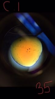

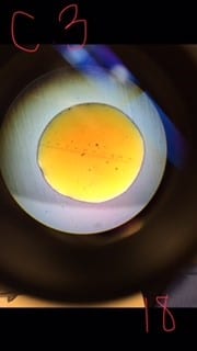
Table 3~ Cell Count Treatment
| Slide | Cell # |
| 1 | 50 |
| 2 | 70 |
| 3 | 30 |


Table 4~ Swim Speed Control
| Control | Time(sec) | Speed(.02/sec) |
| cell 1 | 1.05 | 0.19 |
| cell 2 | 0.93 | 0.22 |
| cell 3 | 0.93 | 0.22 |
| cell 4 | 0.95 | 0.21 |
| cell 5 | 0.93 | 0.22 |
| cell 6 | 0.9 | 0.22 |
| cell 7 | 1.35 | 0.15 |
| cell 8 | 1 | 0.2 |
| cell 9 | 1.21 | 1.21 |
| cell 10 | 1.32 | 1.32 |
Table 5~ Swim Speed Treatment
| Treatment | Time(sec) | Speed(.02/sec) |
| cell 1 | 0.7 | 0.29 |
| cell 2 | 0.76 | 0.26 |
| cell 3 | 0.61 | 0.33 |
| cell 4 | 0.62 | 0.32 |
| cell 5 | 0.53 | 0.38 |
| cell 6 | 0.48 | 0.42 |
| cell 7 | 0.55 | 0.36 |
| cell 8 | 0.19 | 0.19 |
| cell 9 | 0.22 | 0.22 |
| cell 10 | 1.15 | 0.17 |
Storage
All microscopes were unplugged and covered up.
Slides were washed and placed on the paper towel to dry.
The tubes of culture were saved for open lab so they were placed in the tube rack and set next to the flask of culture.
Pipette tips were discarded into the cup.
Pipettes were placed on the stand.
The table was cleared.
Conclusion
This lab was pivotal in our experiment because we started working on our methods and materials section and given the opportunity to expand our knowledge of lab skills. Due to the natural time crunch of our lab, we were expected to work diligently and precisely. This gave us the extra push we needed to dig deeper into our research. We executed the lab skills that we have been practicing with more speed. We also quickened our turn-around speed of going from learning to practicing with the serological pipette and spectrophotometer. All in all this fast paced lab encouraged us to continue with our research even under stressful conditions. These skills can be transferred to many different aspects including studying, working, and even complex thinking.