Megan Hudson                                                                                               April 25, 2019

BIO 1106-22

Lab #14: Poster Presentation and Abstract Submission

Section I: Objective

The purpose of this lab was to edit and submit our final abstract and poster for the CURES Symposium presentation. We also ensured that all metadata was recorded for the soil samples to allow Dr. Adair to pick the most viable sample to send off for sequencing.

Section II: Procedure

1. Vote on CILI-CURE Logo for possible merchandise
2. Record sample identifier, GPS location, tree species, BHD (cm), pH, soil texture, extraction method, DNA concentration, volume, PCR results (+ or -), and soil label on bag into Metadata File Spreadsheet
3. Label DNA tube with AHM22_5Sp19, concentration, and volume of sample
4. Place the tube with a new label into microfuge tube rack
5. Take the remainder of the lab to edit poster and abstract within lab groups.

Section III: Results

Metadata File:

Abstract:

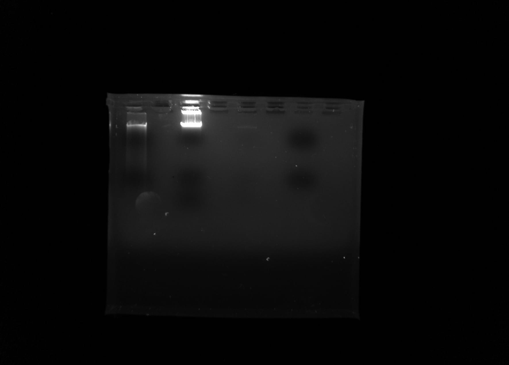
The biodiversity of microorganisms within terrestrial ecosystems is dependent on the viability of the community profile. Soil microbiomes and the influence of eukaryotes within is largely unexplored. The following field experiment analyzes soil collected from the rhizosphere of a Quercus virginiana to attempt to further classify ciliates and understand the diversity of one of the most controversial monophyletic groups, SAR. Metadata regarding soil texture, percent water content, and pH were obtained from each soil sample. The MNH soil sample was identified as sandy loam and KRM and MAA soil samples were identified as sandy clay. The samples were then isolated and eDNA was extracted using silica beads. The eDNA was then cleaned with 80% isopropanol alcohol and primed with an 18S V4 primer to isolate the V4 region of DNA in eukaryotes. The MNH and KRM samples underwent gel electrophoresis to attempt to view bands of DNA and KRM sample was amplified using a polymerase chain reaction (PCR). Results from the PCR amplification were analyzed using the NanoDrop 2000 Spectrophotometer and the MBC C305 UV gel imager. The MNH sample yielded an A260/280 concentration of 1.3 and the KRM sample yielded 1.44, indicating that DNA was present in the sample. Though it was shown that DNA was present, gel electrophoresis images produced no visible bands. These results indicate that soil collected from the rhizosphere surrounding the Quercus virginiana did not contain quantifiable eDNA for eukaryotes, despite ciliates being observed and cultured before soil eDNA was extracted.

Final Poster:

FINAL- Analysis of Soil and eDNA from the Rhizosphere of a Quercus virginiana; Megan Hudson, Madison Ambrose, Kelsi Menzie (1)-2jauozb

Section IV: Where your sample was stored

All soil sample bags were labeled at the beginning of the semester and stored under the fume hood and samples that produced positive PCR and gel electrophoresis results were put into deep freeze.

Section V: Conclusion and Discussion

Posters and abstracts were finalized and submitted so the poster could be printed, and the abstract could be uploaded to the brochure for CURES Symposium next week. Metadata was recorded in the class spreadsheet so samples that are viable enough to send off for sequencing have proper data for future studies. In both the KRM and MNH soil samples, results from the NanoDrop indicated a presence of eDNA, but when we ran our gels and performed PCR, results were negative and did not show a presence of DNA. Since our results were negative for eDNA abundance, most likely our samples will not be sent for sequencing. Although my groups’ samples did not produce positive results, we still were able to establish a methodology for DNA extraction and PCR amplification for future CILI-CURE labs. Moving forward, my group plans to practice presenting our poster so we are prepared for CURES next Friday. As the semester comes to an end, I am grateful for all the research experience and scientific writing skills I have learned in CILI-CURE.

Megan Hudson                                                                                   April 18, 2019

BIO 1106-22

Lab #13: Soil eDNA Metabarcoding Analysis: QIIME 2

Section I: Objective

The purpose of this experiment was to further investigate metabarcoding and to walk through the provided steps to investigate the presence of various ciliate species within the Chelex eDNA sample and the PowerSoil eDNA sample and compare them.

Section II: Procedure

1. Ensure QIIME 2 is downloaded to laptop or desktop computer
2. Download folder provided in Box
3. Activate QIIME 2 by using the command “source activate qiime2-2019”
4. Copy and paste CILICURE _2018 folder after cd command to change to that director
5. Importing sequences as QIIME2 artifact within the cili cure 2018 directory to emp-paired-end-sequences.qza

qiime tools import \

–type EMPPairedEndSequences \

–input-path emp-paired-end-sequences \

–output-path emp-paired-end-sequences.qza

6. Save sample data to a demux.qza file using

qiime demux emp-paired \

–m-barcodes-file sample-metadata.tsv \

–m-barcodes-column BarcodeSequence \

–i-seqs emp-paired-end-sequences.qza \

–o-per-sample-sequences demux.qza \

7. Save demultiplexed visualization to demux.qzv

qiime demux summarize \

–i-data demux.qza \

–o-visualization demux.qzv

8. Feature table frequency and sequence data were saved and reads were denoised using DADA2 stats

qiime dada2 denoise-paired \

–i-demultiplexed-seqs demux.qza \

–p-trunc-len-f 220 \

–p-trunc-len-r 220 \

–o-table table.qza \

–o-representative-sequences rep-seqs.qza \

–o-denoising-stats denoising-stats.qza

9. Feature table visualization was saved to a table.qzv file

qiime feature-table summarize \

–i-table table.qza \

–o-visualization table.qzv \

–m-sample-metadata-file sample-metadata.tsv

10. Visualization was saved to rep-seqs.qzv file

qiime feature-table tabulate-seqs \

–i-data rep-seqs.qza \

–o-visualization rep-seqs.qzv

11. The visualization was saved to denoising-stats.qzv

qiime metadata tabulate \

–m-input-file denoising-stats.qza \

–o-visualization denoising-stats.qzv

12. Phylogenetic tree was created and feature data and phylogeny was saved to aligned-rep-seqs.qza, masked-aligned-rep-seqs.qza, unrooted-tree.qza, rooted-tree.qza

qiime phylogeny align-to-tree-mafft-fasttree \

–i-sequences rep-seqs.qza \

–o-alignment aligned-rep-seqs.qza \

–o-masked-alignment masked-aligned-rep-seqs.qza \

–o-tree unrooted-tree.qza \

–o-rooted-tree rooted-tree.qza

13. Using taxonomic classification program, distinguish between feature table data and create a taxa bar plot

qiime feature-classifier classify-sklearn –i-classifier silva-132-99-515-806-nb-classifier.qza –i-reads rep-seqs.qza –o-classification taxonomy.qza

qiime metadata tabulate \

–m-input-file taxonomy.qza \

–o-visualization taxonomy.qzv

qiime taxa barplot \

–i-table table.qza \

–i-taxonomy taxonomy.qza \

–m-metadata-file sample-metadata.tsv \

–o-visualization taxa-bar-plots.qzv

14. QZV files were dragged and dropped into the Qiime 2 viewfinder
15. Using the taxa-bar-plots.qzv visualization, a Ciliophora group feature ID was copied and pasted into the finder for the rep-seqs.qzv to BLAST.
16. After blasting the identified sequence, possible identifications were linked and investigated.
17. Computers were shut down and all QTM were answered

Section III: Data and Observations

Taxa-bar-plots.qzv
Phylogenetic Tree for Dexiotricha

Within the Alveolata supergroup, 15 Ciliophora groups were present, some unidentified, in the PowerSoil and the Chelex eDNA samples. Hypotrichia was identified in both samples, 16.600% in Chelex sample and 0.417% in PowerSoil sample. Peniculia was identified in both samples, 0.221% in Chelex and 10.330% in PowerSoil. Scuticociliatia was identified in both samples, 9.845% in Chelex and 0.225% in PowerSoil. Spirotrichea was identified in both samples, 4.283% in Chelex and 1.668% in PowerSoil. Colpodida was identified in both samples, 2.119% in Chelex and 1.380% in Power Soil. Heterotrichea was only in Chelex, being 3.223%. Cyrtophoria was only in Chelex, being 1.810%. Platyophryida was identified in both samples, 0.353% in Chelex and 0.321% in Power Soil. Nassophorea was only present in Chelex, being 0.618%. Hymenostomatia was only present in Chelex, being 0.397%. Haptoria was only present in Chelex, being 0.265%. Haptoia was only identified in the Power Soil and was 0.265%. Litostomatea was only identified in the Power Soil, is 0.160%. Oligohymenophera was only identified in the Chelex sample, is 0.132%. Comparing both samples, most ciliate groups were either present in both samples or was only in the Chelex eDNA sample. This could be due to better DNA extraction protocol in the Chelex sample.

After performing BLAST, I identified a percentage of similarity to Dexotrichia within the eDNA. An article, Morphological reports on two species of Dexiotricha (Ciliophors, Scuticociliatia), with a note on the phylogenetic position of the genus, was used to further investigate the morphological characteristics of the Dexiotricha genus and species within. The Dexotricha genus contains both Ciliophora and Scuticociliatia species. Dexotricha has been proposed as a monophyletic genus, but questions surround its familial assignment since it has not been subjected to molecular phylogenetic analysis to make a for certain connection. Scutiociliates are identified as free-living organisms commonly found in limnetic and marine environments. Dexiotricha is defined to have a ‘scuticobuccokinetal’ pattern, distinct ring-like granules, and the contractile vacuole (excretory pore) has been previously reported to be located equatorially. Since morphological observations were not made and this specific species is usually water-borne, I am not for certain that this eDNA identification can be made in a soil eDNA sample.

Section IV: Where your sample was stored

Computers were shut down and all data was saved to the CILI CURE_2018 folder and was uploaded onto Module 13 on Canvas.

Section V: Conclusion and Future Steps

This lab allowed students to become familiar with the QIIME 2 program and use the provided codes for the Moving Tutorials used last week and use the visualizations to possibly identify ciliate eDNA found in the Chelex and the PowerSoil samples. Using the QIIME 2 Program allowed us to analyze the relative abundance of different types of supergroups and ciliate species present in our eDNA samples and analyze the diversity present within the reads collected from last year’s samples. Using the visualizations allowed us to BLAST a read with high abundance and analyze its similarity to other identified ciliates. We further investigated the metadata and characteristics of possible identified ciliates on PubMed, which also allowed us to witness the many identifications that aren’t already identified. This could result in our samples actually having ciliate eDNA that hasn’t been investigated, meaning that we could have found a new species! Moving forward, we hope to use the CyVerse platform to run the QIIME program alongside the Jupyter Notebooks and orient our eDNA reads. This will allow us to analyze the biodiversity of supergroups and ciliate species present in the samples and hypothesize how the metadata and the metagenomics are interconnected and might influence each other.

Megan Hudson                                                                                               April 11, 2019

BIO 1106-22

Lab #12: UNIX and Setting Up the System

Section I: Objective

The purpose of this lab was to follow the Moving Tutorial steps and continue working with the QIIME 2 program so we are comfortable with the terminal application and using code to analyze our own eDNA V4 reads.

Section II: Procedure

1. Ensure QIIME 2 is downloaded
2. Adair will give background information about FASTA and FASTQ and reviewed information regarding Next-Generation Sequencing and what we will be doing in the weeks to come
3. Activate QIIME 2 source
4. Type “pwd” into the terminal to allow data to be saved under the print-working directory named qiime2-moving-pictures-tutorial
5. Insert Path Bar using View and the Finder to retrace steps
6. Open Sample Metadata on Moving Pictures Tutorial
7. Paste wget code into the terminal to download sample metadata

wget \

-O “sample-metadata.tsv” \

“https://data.qiime2.org/2019.1/tutorials/moving-pictures/sample_metadata.tsv”

8. Paste to wget code to download practice sequences provided

wget \ -O “emp-single-end-sequences/barcodes.fastq.gz” \  “https://data.qiime2.org/2019.1/tutorials/moving-pictures/emp-single-end-sequences/barcodes.fastq.gz”

Paste Qiime Tool Import code to create a qza file

wget \  -O “emp-single-end-sequences/sequences.fastq.gz” \  “https://data.qiime2.org/2019.1/tutorials/moving-pictures/emp-single-end-sequences/sequences.fastq.gz”

8. Demultiplex code is pasted into the terminal to distinguish samples

qiime demux emp-single \  –i-seqs emp-single-end-sequences.qza \  –m-barcodes-file sample-metadata.tsv \  –m-barcodes-column BarcodeSequence \  –o-per-sample-sequences demux.qza

9. Generate a summary of demultiplexed results and save visualization as a qzv file by pasting the code into the terminal

qiime demux summarize \  –i-data demux.qza \  –o-visualization demux.qzv

10. Drag and drop the qzv file into QIIME 2 View website to create a visual interactive quality plot
11. Look at quality scores to determine which base pairs to cut out
12. DADA 2 and DEBLUR will denoise the samples and ensure the sample is cut after 0 to 120

qiime dada2 denoise-single \  –i-demultiplexed-seqs demux.qza \  –p-trim-left 0 \  –p-trunc-len 120 \  –o-representative-sequences rep-seqs-dada2.qza \  –o-table table-dada2.qza \  –o-denoising-stats stats-dada2.qza

13. Copy and paste QIIME Metadata Tabulate code to create an organized spreadsheet of the data

qiime metadata tabulate \  –m-input-file stats-dada2.qza \  –o-visualization stats-dada2.qzv

14. Drag and drop stats-dada2.qzv into QIIME 2 View https://view.qiime2.org/visualization/?type=html&src=49f1655b-cf8c-4afe-9897-2b838c9d4d7f
15. Rename qzv file to table.qza

mv rep-seqs-dada2.qza rep-seqs.qzamv table-dada2.qza table.qza

16. Output visualization and put metadata attached to it by converting the table into a qzv file

qiime feature-table summarize \  –i-table table.qza \  –o-visualization table.qzv \  –m-sample-metadata-file sample-metadata.tsvqiime feature-table tabulate-seqs \  –i-data rep-seqs.qza \  –o-visualization rep-seqs.qzv

17. Get a database that will be used to analyze taxonomy results

wget \  -O “gg-13-8-99-515-806-nb-classifier.qza” \  “https://data.qiime2.org/2019.1/common/gg-13-8-99-515-806-nb-classifier.qza”

18. Convert taxonomy file into a qzv file

qiime feature-classifier classify-sklearn \  –i-classifier gg-13-8-99-515-806-nb-classifier.qza \  –i-reads rep-seqs.qza \  –o-classification taxonomy.qza qiime metadata tabulate \  –m-input-file taxonomy.qza \  –o-visualization taxonomy.qzv

19. Drag and drop taxonomy qzv file into QIIME 2 View to analyze the confidence level of the samples present
20. Create taxa bar plot

qiime taxa barplot \  –i-table table.qza \  –i-taxonomy taxonomy.qza \  –m-metadata-file sample-metadata.tsv \  –o-visualization taxa-bar-plots.qzv

21. Drag and drop taxa bar plot qzv file from the Finder into QIIME 2 View to analyze taxa levels and observe diversity present. Levels present are clean samples with high confidence levels.
22. Ensure all files are saved in qiime2-moving-pictures-tutorial and analyze provenance steps

Section III: Data and Observations

Demultiplexed File	Demultiplexed Quality Plot	Taxa Bar Plot Visualization	Soil Metadata Spreadsheet

Section IV: Where your sample was stored

Computers were shut down, and all data was saved to the qiime2-moving-pictures-tutorial file on my personal laptop.

Section V: Conclusion and Future Steps

This lab allowed students to become familiar with the QIIME 2 program and begin using the codes for the Moving Tutorial.  After our genomes are sequenced, we can use the QIIME 2 program to analyze large sums of data and allow us to organize it properly for publishing. Using the QIIME 2 Program can allow us to analyze the relative abundance of different types of phyla present in our eDNA samples and analyze the diversity present within the various reads from the V4 region collected from the sample. We can use clean, accurate data with a high confidence rate to create visualizations and figures that can be used for conclusions and publishing. Moving forward, we hope to use the CyVerse platform to run the QIIME 2 program alongside the Jupyter Notebooks and orient our eDNA reads. The Jupyter Notebooks will allow us to compare and contrast the eDNA reads from the collected samples from our class and identify the common markers between the reads. The CyVerse platform will allow all our data to be uploaded for both our class and other research projects. Using these programs and visualizations will allow us to analyze the biodiversity present in the samples and hypothesize how the metadata and the eDNA influence each other.

Megan Hudson                                                                                               April 4, 2019

BIO 1106-22

Lab #11: Poster Presentations (SW) Cloud Computing and Jupyter Notebooks

Section I: Objective

The purpose of this lab was to start the process of metagenomic analysis and install the QIIME 2 Program. Becoming familiar with this program will allow us to analyze the reads collected from eDNA samples.

Section II: Procedure

1. Open Terminal
2. State commands and practice using the terminal
3. Open and follow QIIME Installation Instructions
4. Download Miniconda 64-bit (pkg installer)0 for your use only
5. Close and reopen terminal
6. Once downloaded, type “conda update conda”
7. Type conda install wget
8. Type “Y” to proceed with updates
9. Install Miniconda macOS/OS X (64-bit) by copying and pasting “wget https://data.qiime2.org/distro/core/qiime2-2019.1-py36-osx-conda.yml conda env create -n qiime2-2019.1 –file qiime2-2019.1-py36-osx-conda.yml”
10. Allow the program to completely download
11. Type “Y” to activate the environment
12. After the download is complete, begin working through the moving pictures tutorials

Section III: Results and Observations

Learned Commands:

Is= list content

Cd= change directory

Say “Sic Em Bears”

Cd-/Documents

Section IV: Conclusion and Future Steps

Becoming familiar with the QIIME 2 Program will better prepare us for analyzing large sums of data and allow us to organize it properly for publishing. Using the QIIME 2 Program can allow us to analyze the relative abundance of different types of ciliates present in our eDNA samples and analyze the diversity present within the various reads collected from the sample. Moving forward, we hope to use the CyVerse platform to run the QIIME program alongside the Jupyter Notebooks and orient our eDNA reads. This will allow us to analyze the biodiversity present in the samples and hypothesize how the metadata and the eDNA influence each other.

Megan Hudson                                                                                   March 28, 2019

BIO 1102-22

Lab #10: Next Generation Sequencing and Metabarcoding

Section I: Objective

The purpose of this lab was to learn about the process of Next-Generation Sequencing and comprehend why we are using Illumina flow cells to analyze eDNA sequences.

Section II: Procedure

1. Make CyVerse Account
2. Aadil and Dr. Adair explained the process of illumina sequencing and what the next five weeks are going to hold in the lab
3. Order steps of Illumina sequencing with a partner in the Card Game
4. Draw out the steps of Illumina sequencing on QTM
5. Answer questions on QTM regarding what parts of the procedure means
6. Draw flow chart explaining what we have done in the lab thus far from purifying eDNA to metabarcoding

Section III: Results and Observations

Illumina Sequencing:

Step 1: Break up genomic DNA into more manageable fragments by using enzymes or by PCR amplification
Step 2: Tag DNA fragments with short sequences of DNA (adaptors)
Step 3: Denature double-stranded molecules into single-stranded molecules that have adaptor and primer binding site—incubate fragments with NaOH
Step 4: Attach DNA fragments to flow cell through complementary binding of the adaptors to the Oligos (primers) on the surface of the flow cell
Step 5: Replicate DNA attached to the flow cell to form small clusters of DNA with the same sequence
Step 6: Unlabeled nucleotide bases and DNA polymerase are added to lengthen and join the DNA strands attached to the flow cell
Step 7: Double-stranded DNA is broken down into single-stranded DNA using heat, leaving several million sense clusters of identical DNA sequences
Step 8: Primers and fluorescently labeled terminators are added to the flow cell
Step 9: Primer attached to the DNA being sequenced
Step 10: DNA polymerase binds to the primer and adds the first fluorescently- labeled terminator to the new DNA strand. Once a base has been added no more bases can be added to the strand of DNA until the terminator base is cut
Step 11: Lasers are passed over the flow cell to activate the fluorescent label on the nucleotide base. Fluorescence is detected by a camera and recorded on a computer—each terminator base gives off a different color
Step 12: Fluorescently labeled terminator group is then removed from the first base the next fluorescently labeled terminator group can be added alongside. The process continues until millions of clusters have been sequenced

Section IV: Where your sample was stored

Computers were shut down after use, cards from the game were returned to Dr. Adair, and purified eDNA sample collected several weeks ago is still being stored in the freezer at -20 degrees Celsius.

Section V: Conclusion and Future Steps

This lab allowed students to understand the meaning behind Illumina sequencing and how it applies to what we are hoping to accomplish moving forward for the next 5 weeks in the lab. Illumina sequencing will allow our groups to amplify the eDNA sequences using PCR amplification, tag the specific nucleotides within the sample and observe them under fluorescent light to differentiate between the bases in the millions of DNA clusters we are hoping to sequence. Moving forward, we hope to use the CyVerse Cloud computing resource to analyze our sequence and establish a collection of eDNA data for the Baylor campus. Metagenomics and metabarcoding are extremely important to biological research and gaining experience and tools in this field will better prepare students for a career in the sciences. I am looking forward to poster presentations and to learning more about the field of metagenomics and how it will help us to connect the microscopic to the macroscopic being the eDNA sequences to the overall terrestrial microbiome.

Megan Hudson                                                                                                           3/21/19

BIO 1106-22

Lab #9: Poster Presentations

Section I: Objective

The purpose of this lab was to present the rough draft of our poster and gather feedback. We can use the feedback and converse with our groups to improve and make any needed changes for the final draft of the poster.

Section II: Poster

 BIO 1106 Poster Presentation-1c6y94y

Section III: Procedure

1. Present Poster
2. Gain feedback from Dr. Adair, Aadil and Kaitlyn
3. Converse and alter poster according to feedback
4. Grade other group’s posters
5. Gain ideas of what the “ideal” final draft needs to look like
6. Log out of the computer

Section IV: Critiques and Changes Made

1. Tree Identification Data
2. Change color scheme and title
3. Delete oak wilt from the introduction
4. Alter captions to better suit the scope of research
5. Conclusions and Future Steps need to include sequencing and ciliate biodiversity inferences
6. Explain why we did not have viable DNA samples and how different environmental factors could have affected DNA concentration by referring to soil metadata
7. Explain why both used DNA samples had positive nanodrop results but negative gel electrophoresis results

Megan Hudson                                                                                                March 7, 2019

BIO 1106-22

Lab #8: PCR Results/ Scientific Poster Design

Section I: Objective

The purpose of this lab was to perform gel electrophoresis on our PCR amplified DNA samples and determine if an adequate amount of DNA is present to send off to be sequenced. We also began designing our research poster and outlining the separate sections.

Section II: Procedure

1. Obtain 1.5% Agarose gel that had been previously prepared
2. Obtain 25 ul PCR amplified DNA sample and 25 ul control sample
3. Place gel in electrophoresis chamber and cover up to brim with 1X TAE loading buffer,
4. Load 10 ul of designated sample into the assigned lane
5. Pipette 5 ul of provided DNA 1kb ladder sample
6. Run gel at 100 V for 30 minutes
7. Go to A305 Computer Lab and complete BIO 1106 Midterm
8. Begin poster design

Section III: Results and Observations

Gel Electrophoresis:

Poster Design	Copy of CILICURE Poster (1)-rodzpb
Gel Figure

Section IV: Where your sample was stored

Micropipettes and gloves were disposed of, and all contaminants were bleached and cleaned. DNA samples and 1 kb ladder samples were placed back into the refrigerator. Lab station was cleaned, and the computer was shut off after use.

Section V: Conclusion and Future Steps

Performing gel electrophoresis on our purified and amplified sequences allowed us to verify the orientation and purity of the DNA within the samples. This verification will allow us to determine which extracted DNA samples are worth sending off to be sequenced. We began the poster design that we are preparing for the CURE presentation. Our poster will consist of the background information regarding the experimental design, methods and procedures, results, and discussion and conclusion. We hope to correlate our results to the overall soil biodiversity and environmental factors that affect the overall balance of the ecosystem. In the end, our results will contribute to the under-researched field of soil microbiomes and will hopefully assist in finding a solution to the growing problem of oak tree wilt.

Megan Hudson                                                                                                           2/28/19

BIO 1106-22

Lab #7: PCR Amplification

Section I: Objective

The goal of this lab was to prepare our purified eDNA for Polymerase Chain Reaction (PCR) amplification using V4 Ribosomal primers and begin to plan our research poster set-up and design.

Section II: Procedure

1. Using Purified DNA Sample Nanodrop Concentration, calculate the amount of DNA template needed to make a 25 ul total volume
2. If calculated DNA template is too small to pipette, use a 1:10 dilution and then calculate the volume of Soil DNA
3. Subtract the amount of 2X master mix, DNA template and primers (10 uM) from 25 total ul to solve or amount of sterile water needed
4. Clean lab table with 10% bleach to create an aseptic environment and use gloves for the remainder of the experiment to avoid DNA contamination
5. Obtain eDNA sample, sterile water, and primers from the iced cooler
6. Obtain 2 tubes of the 2X Master Mix (Taq polymerase, buffers, and nucleotides) from the refrigerator
7. Label green nanotubes containing 12.5 ul of the 2X master mix as control or Soil DNA tube
8. Pipette 1 ul of the 10 uM 18S V4 primer into the green control nanotube
9. Pipette 11.5 ul water into the tube in 2 increments (5 ul then 6.5 ul)
10. Create a diluted DNA sample by adding 9 ul sterile water to 1 ul eDNA in a new centrifuge tube
11. Pipette 3.065 ul of the diluted DNA sample into the DNA nanotube
12. Pipette 1 ul 10 uM 18S V4 primer and 8.435 ul sterile water into the tube
13. Place labeled tubes into the thermocycler and record tube numbers
14. Dispose of empty tubes and return water and primers to the cooler
15. Begin to design scientific poster over the research conducted from this semester

Section III: Results and Observations

Purified DNA Sample Nanodrop (New) 2/22/29:

Tube Numbers:

Control = 11E

Soil DNA = 12E

Section IV: Where your sample was stored

Empty tubes used for DNA sample dilution were disposed of, and all used tubes of primers and water were returned to the cooler. PCR samples were placed into the thermocycler. Lab stations were cleaned.

Section V: Conclusion and Future Steps

Using our soil eDNA samples mixed with primers, Taq Polymerase, buffers, nucleotides, and sterile water, we will perform polymerase chain reaction amplification. The thermocycler will automatically alter the temperature to allow the DNA sequence to denature, anneal, and elongate over about 21 cycles. After the PCR amplification is completed, we can distinguish whether any DNA was reproduced by running the PCR sequences on a new agarose gel. This will determine whether the sample was viable and whether it is worth sending off to be sequenced. We began to design our scientific poster that will be presented regarding our results for the Gel Electrophoresis, PCR Amplification, and DNA sequencing and how these results relate to the biodiversity of the soil.

Megan Hudson                                                                                   February 21, 2019

BIO 1106- 22

Lab #6: Gel Electrophoresis and DNA Analysis

Section I: Objective

The purpose of this lab was to perform gel electrophoresis and observe the DNA bands within the gel. Using these observations will help us conduct research on the soil ciliate biodiversity by analyzing the DNA sequence of the soil environment.

Section II: Procedure

1. Start by practicing the technique of pipetting the 1 X loading buffer into the gel with Dr. Adair
2. Be sure to have gloves on to prevent contamination with the Ethidium Bromide (since its a carcinogen)
3. Place gel in the electrophoresis chamber in the correct orientation with the wells at the negative end of the chamber
4. Pour 1X TAE running buffer over the gel to completely submerge the gel
5. Assign wells to each DNA sample and DNA mass standard and draw a picture of what sample will go where.
6. Pipette 9 ul of the DNA sample and 1 ul of the 10x loading buffer into the small green nano-centrifuge tube to make a 10 ul total 1x buffer
7. Centrifuge the 10 ul total 1x buffer to fully mix the DNA with the buffer
8. Pipette 10 ul of the purified DNA sample from Group 6 into Lane 1
9. Pipette 10 ul of the purified DNA sample from Group 5 in Lane 7
10. Load 5 ul DNA mass standard 1 (500 ng) in Lane 3
11. Load 5 ul of the DNA mass standard 2 (15 ng ) in Lane 5
12. Place top on the chamber and attach electrodes to the positive and negative ends
13. Run the gel at 100 volts for approximately 20 minutes
14. Take gel to the lab, place on the UV screen, and run the computer analysis program to visualize the DNA bands
15. The ethidium bromide intercalated within the gel promoted the bands to fluoresce under UV light
16. Using DNA mass standards, the bands of the DNA can be compared to the width and pigmentation of the standard to give an approximation of the mass of the fragments
17. In the lab, we also performed absorbance tests over our purified DNA sample using the Nanodrop Spectrophotometer
18. A 2 ul sterile water sample was placed on the optical surface to serve as a blank measurement
19. A 2 ul drop of the purified DNA sample was placed on the optical surface
20. The concentration and purity ratios were calculated
21. The 260/280 ratio and the 260/230 ratio were analyzed
22. The gel was returned to the refrigerator, and all used utensils were properly disposed of
23. Work station was cleaned

Section III: Results and Observations

Gel Mock Up:

Lane 1	Lane 2	Lane 3	Lane 4	Lane 5	Lane 6	Lane 7	Lane 8	Gel
Group 6 DNA	—	DNA Mas STD 1	—	DNA Mass STD 2	—	Group 5 DNA	—

Gel under UV Light:

DNA Sample Nanodrop Spectrophotometer Analysis:

Section IV: Where your sample was stored:

The agarose gel cast was stored in the refrigerator, and the remainder of the purified DNA sample was stored in the freezer at -20 degrees Celsius.

Section V: Conclusion and Future Steps

In this lab we performed gel electrophoresis by adding our purified DNA samples to the gel and using a battery to pull the negative charge of the DNA towards the positive end of the battery, creating bands of DNA based on the fragment size. When loading the 500 ng mass standard 1, 50 ul were pipetted instead of 5 ul, making it a 5000 ng solution and possibly skewing our comparison results. The Ethidium Bromide intercalated within the bands of the DNA, in a way mimicking a base pair. Placing the gel under a UV light allowed the bands of the DNA to fluoresce and allowed us to see the relative size and orientation of the DNA sequence. Unfortunately, our DNA sample did not produce any visible bands, therefore, our group has to perform DNA purification and run the gel again in open lab to hopefully produce better results. Since the smaller fragments will travel through the micro- inconsistencies to the bottom of the gel and the larger fragments will remain at the top of the gel, we should be able to observe the variation among the different soil sample’s DNA sequence. Since the goal of this lab is to develop research in soil ciliate biodiversity, observing and sequencing the DNA of the soil will allow us to better develop the community profile of the ciliates living within our soil samples.

Megan Hudson                                                                                               February 14, 2019

BIO 1106-22

Lab #5: DNA Extraction

Section I: Objective

The goal of this lab was to extract DNA from our crude eDNA samples from our soil and use DNA purification and gel electrophoresis to sequence and analyze the DNA fragments. This lab involved the setting up of the gel and purifying the DNA sample so that in a later lab we will be able to perform the gel electrophoresis and PCR sequencing.

Section II: Procedure

DNA Purification

1. Retrieve crude eDNA samples and add sterile water to make a 1 ml total liquid sample and transfer this liquid sample to a 15 ml conical tube.
2. Add 2 ml of DNA resin (at 37 degree Celsius)
3. Set up a column onto a syringe barrel and place onto the vacuum filtration system
4. Transfer half of the liquid sample into the syringe barrel in 150 ul increments. After all of the liquid has been pulled through, add the remainder of the sample.
5. Begin washing and purification process by adding 2000 ul 80% isopropanol and use the negative pressure of the vacuum filtration system to pull the liquid through.
6. Repeat washing process 2 more times (6000 ul total)
7. Remove the column from the barrel and place the column into a clean 1.5 ml Eppendorf tube
8. Spin tube at 8000 x g for 5 minutes to remove any residual isopropanol
9. Put tubes into the 80 degrees Celsius heat block and incubate for 1 minute
10. Transfer column into a new Eppendorf tube and pipette 50 ul sterile distilled water (heated to 80 degrees Celsius) into the column
11. Incubate for 1 minute
12. Spin sample in the centrifuge at 8000 x g for 1 minute
13. Place tubes into the freezer at -20 degrees Celsius
14. Discard column and any other remaining used tubes into the biohazard trashcan

Agarose Gel Electrophoresis

1. Use 4 ml of the 10x TAE stock solution and 36 ml DI water to create 40 ml of 1xTAE solution (C1V1=C2V2)
2. The solution was transferred to a conical vile
3. Weigh out 4 grams of the Agar Powder and add to a 125 ml Erlenmeyer flask
4. Pour the 40 ml of the 1xTAE solution into the Erlenmeyer flask to create a 1% Agar solution
5. Microwave flask for 1 minute (Power 7)
6. Mix the solution thoroughly until the solution is clear and small bubbles come off the bottom when gently swirled
7. Pipette 2 ul Ethidium Bromide into the flask
8. Pour 1xTAE and Agar solution into the gel cast
9. Wait about 30 minutes for the gel to cool
10. After the gel is solidified, pour 1xTAE over the gel, creating a thin top layer that completely covers the gel and up to the brim of the mold
11. Label cast and place into a plastic bag
12. Put gel cast into the refrigerator to store for a week

Section III: Observations

Throughout this procedure, we were able to observe the very tedious process of DNA extraction and how little the extraction process yields from the original 1 ml sample. Our crude eDNA lysate was a dark brown color, and after the vacuum filtration removed all the impurities, the sample was clear. The setup of the agarose gel involved harsh carcinogens and resulted in an iridescent jelly-like substance.

Section IV: Where your sample was stored

All used utensils, tubes and instruments were disposed of in the biohazard trashcan. The agarose gel cast was stored in the refrigerator, and the purified DNA sample was stored in the freezer at -20 degrees Celsius.

Section V: Conclusion and Future Steps

This lab involved the purification of our crude eDNA lysate to use in our gel to analyze the DNA profile of our soil and differentiate between the fragment sizes based on their orientation in the gel. In the next lab, we will perform gel electrophoresis by adding our purified DNA to the gel and observing the bands under a UV light. The gel electrophoresis process involved the addition of the Ethidium Bromide to allow the gel to illuminate under the UV light to better visualize the fragments in fluorescent light. Adding a positively charged battery at the end of the gel will that pull the negatively charged DNA towards it. Since the smaller fragments will travel through the micro- inconsistencies to the bottom of the gel and the larger fragments will remain at the top of the gel, observation of the gel should give us a visual description of the DNA sequence.