Christina Clark

November 5, 2018

Lab 12 Discovering Ciliates

OBJECTIVE

The purpose of lab 12 was to build the knowledge of Ciliate structure, function, and taxonomy by observing soil ciliates in order to identify them by their morphological characters. We also were looking at the classes of ciliates and their relation to the tree of life. This is important to know the diversity of ciliates and their role in the environment.

PROCEDURE

Soil Sample:

1. Take 4ml of the original soil sample and place in a Falcon tube.
2. Fill the Falcon tube until the volume reaches the 10 ml mark.
3. Place on vortex for 10 seconds.
4. Put one drop of dispersing agent into the mixture.
5. Place on vortex for 10 seconds.
6. Label the tube and store.

Unknown Soil Ciliate Investigation

1. Take the Petri dish of the rehydrated soil sample.
2. Add 20 ml sample to a flat slide and observe under a compound microscope. Confirm that there are ciliates in the sample.
3. Add 10 ml of methyl cellulose to the sample and mix by slowly pipetting up and down.
4. Record observations and take a picture.

RESULTS

They are clear and small. They move slowly and change directions often.

STORAGE

The Falcon tube was stored at room temperature; sitting upright in a test tube rack. The bag of soil and the Petri dish were both stored at room temperature inside the lab.

CONCLUSION

I was only able to find two of the same ciliates in my sample. They are very small and clear, and I was unable to observe enough of their behavior to be able to identify them. They were ovular and moved slowly; changing directions often. However, I was able to take a picture of them.

FUTURE STEPS

In the future, I would like to be able to observe how these ciliates benefit or hinder our environment and understand their purpose to our ecosystem.

Christina Clark

October 25, 2018

Lab 10: Writing Analysis

Title and Authors:

It is important to include this because it acknowledges the work you and your group have accomplished. Make sure your title is exactly what the lab is about. Do not make the title too general. This allows the reader to know specifically what the main idea of the report is.

Abstract

This is a brief summary of the paper that goes over what was researched, hypothesis, methods, results and conclusion. This is only a summary; the detail will come later in the paper. Abstracts help the reader to understand quickly what the papers purpose is.

Introduction:

The introduction gives background information on the experiment. This may include data that is already known which allows you to explain the relevance of the experiment and how this information will be beneficial to the scientific field.

Materials and Methods:

The Material and Methods describe the procedure of the lab. It is important to be precise during this so that if someone else were to recreate the lab they would be able to follow the same procedure and come up with the same results.

Results:

The results give the reader a visual representation of the data, along with numbers that will reveal the answers to the authors hypothesis. The data should be organize so that it easy to understand from a readers perspective, especially if they did perform the experiment.

Discussion:

This is  where the authors analyze the data and make conclusion on whether to reject the null hypothesis or not. This is also where the author will discuss the implications of the experiment and report any sign of unexpected or ambiguous results.

Christina Clark

October 18, 2018

Lab 9: Charts and Graphs

OBJECTIVE

The objective of this lab is to compare the growth of the control group to the growth of the treatment group. We will become more familiar with excel and calculate the standard deviation and forming figures for a visualization of the data.

PROCEDURE

Cell Count

1. Using the data from your descriptive statistics for your cell counts, select the mean and standard error.
2. Using your data (including the starting cell concentration), make a bar chart.
3. Add axis labels and a title. Select the chart and under the tab chart design, click Add Chart Element and select Axis Titles and Chart Title.
4. Add Standard Errors Bars. Click on the “Custom” button under “Error Amount” and click on the “Specify Value” button. Then small Custom Error Bars dialog box will then appear asking you to specify the values of your error bars.
5. Add an asterisk for designating statistical significance.

Optical Density

1. Subtract the PPT + Twine Extract from the Treatment values.
2. Place these values into a column and run a descriptive statistics test on them.
3. Run a descriptive statistics test on the Control data values.
4. Use the means and standard errors from the two descriptive statistics tests to make a new chart for the control and treatment values.
5. Using the means, make a bar graph.
6. Add axis labels and a title. Select the chart and under the tab chart design, click Add Chart Element and select Axis Titles and Chart Title.
7. Add Standard Errors Bars. Click on the “Custom” button under “Error Amount” and click on the “Specify Value” button. Then small Custom Error Bars dialog box will then appear asking you to specify the values of your error bars.
8. Add an asterisk for designating statistical significance.

DATA

CONCLUSION

By observing the data my group was able to conclude that the treatment grows faster than the control. We did this by going into excel and using it to calculate the numbers in order to for

m data. Then compared the data to see the difference in to control and treatment group.

FUTURE STEPS

In the upcoming labs we will be able to hypothesize how the growth of the treatment affects our environment. We will also compare our data with other groups and begin writing our lab reports.

Christina Clark

October 11, 2018

Lab 8: Data Analysis

OBJECTIVE

Today’s lab will focus on the analysis of data. Students should know how to retrieve data and collaborate effectively by understanding the value of data and accurately interpret it to find correct results. Based off of the previous week’s experiment, student combined data collaboratively on one Excel spreadsheet. With the given inquiry students found the Descriptive Statistics, Histograms, F-Test, and T-Test of their cell counts and assigned assay. After this, student interpreted the results to make a sound judgement on whether to accept or reject the null hypothesis. A null hypothesis is a hypothesis that there is no significant difference between specified populations, and that any observed difference being die to sampling or experimental error.

PROCEDURE

Descriptive Statistics

1. Make sure you have access to the ToolPak for Excel. These tools are free and can be added to your Excel software if they are not already included.

• Mac Users: Tools/Excel Add-In/ToolPak. The Data Analysis Box is now on the Data Toolbar or under the Tools Menu.
• PC Users: File/Options/Add-Ins/Analysis ToolPak/Go; Check the Analysis ToolPak box/OK.

On the Data tab, in the Analysis group, you can now click on Data Analysis.

2. Organize your data in an Excel Spreadsheet by putting all the data in separate columns giving it its respected header.
3. Open the Data Analysis tool under the Data tab. Select Descriptive Statistics and click OK.
4. Enter the range of the data you want to be analyzed. Then click the box that is marked Summary Statistics and click OK.
5. Do this for each column of data including Control/Treatment cell counts and the data from the vacuole assay.
6. Copy and paste the data analysis onto one sheet in order to be able to compare the data without clicking between tabs.

Histograms and Normal Distribution

1. On the Data tab, in the Analysis group, click Data Analysis. Select Histogram and click OK.
2. Select the Input Range for your data.
3. Click in the Bin Range box and select the cells that include the bin numbers.
4. Click the Output Range Option button, click in the Output Range box and select the cell where you want the output to be sent.
5. Check the box marked Chart Option and click OK.
6. Transfer all the data to the data sheet.

The F-Test and Variance

1. Open the Data tab, in the Analysis group, click Data Analysis.
2. Select F-Test Two-Sample for Variance and click OK.
3. Click in the Variable 1 Range box and select the range of your control measurements.
4. Click in the Output Range box and select a cell for the output. Click OK.

The t-Test

1. On the Data tab, in the Analysis group, click Data Analysis.
2. Select the correct t-Test for your data. (Either Paired Two Sample for Means, Two-Sample Assuming Equal Variances) Click OK.
3. Click in the Variable 1 Range box and select the range for your Control data.
4. Click in the Variable 2 Range box and select the range for your Treatment Data.
5. Click in the Hypothesized Mean Difference box and type 0.
6. Click the Output Range box and select a cell for your Output. Click OK.

DATA

CONCLUSION

Descriptive Analysis:

The descriptive analysis allows us to get a quick overview of the Mean and Range for each data set.

Histogram Control Cell Count:

Our main interest in the histogram is to visualize the distribution of the data. The distribution of the data varies by increasing, decreasing, and then increasing again as you read the data from left to right. This is not a normal curve to this data most likely due to the small sample sizes. However, we will still use the t-Test for analysis regardless of the distribution.

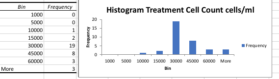
Histogram Treatment Cell Count:

The distribution of data, in this case, is a normal curve due to its bell curve like shape; increasing and then decreasing from left to right.

Histogram Control Vacuole Formation:

The distribution of data, in this case, is an abnormal curve due to its constant decrease from left to right.

Histogram Treatment Vacuole Formation:

The distribution of data, in this case, is normal due to its increase and the decrease from left to right.

f-Test: Two-Sample for Variances Control and Treatment Cell Count:

If F>F Critical one-tail, we reject the null hypothesis that the variances of the two populations are equal. Therefore, 4.01>1.75 leading to the conclusion that the variances of the populations are not equal causing us to reject the null hypothesis.

f-Test: Two-Sample for Variances Control and Treatment Vacuole Formation:

If F<F Critical one-tail, we accept the null hypothesis that the variances of the two populations are equal. Therefore, 1.09<1.31 leading to the conclusion that the variances of the populations are equal causing us to accept the null hypothesis.

t-Test: Two-Sampling Assuming Unequal Variances Control and Treatment Cell Count:

If -t Critical>t Stat>t Critical two-tail, we reject the null hypothesis and assume that there is a significant difference between the two means. In this case, -1.96<3.02>1.96. Therefore, we do not reject the null hypothesis.

t-Test: Two-Sampling Assuming Equal Variances Control and Treatment Vacuole Formation

If -t Critical>t Stat>t Critical two-tail, we reject the null hypothesis and assume that there is a significant difference between the two means. In this case, -1.9<3.01>1.97. Therefore, we do not reject the null hypothesis.

FUTURE STEPS

In future labs, we hope to further analysis our data collaboratively to determine what the cause of variance is between our control and treatment groups. By using that data we will be able to form a hypothesis as to how our experiment will affect the survival rate and behavior the twine juice will have on the Tetrahymena.

Christina Clark

Lab 7: Hay Bailing Twine Challenge Preparation, Vacuole Assay

Objective

The purpose of this lab was to continue the preparation of the Hay Bailing Twine Challenge by observing the difference between the treatment and control. The treatment is pure Tetrahymena and the control was Tetrahymena and the PPT combined. Throughout this past week, Dr. Adair also furthered the progress of the experiment. (The additional steps done outside of class will be listed below under procedures). Along with the treatment/control observation, there was also additional focus on the vacuole assay. We performed this assay last week but improved it to get better results.

Procedure

Treatment/Control Groups

1. Each flask has 50ml of culture. Swirl the flask before pipetting.
2. Label the tubes. One for treatment and the other for control. Make sure to keep the tubes covered.
3. Transfer 4ml of the treatment and control into sterile glass tubes using serological pipettes.
4. Take 3 2ul drops of the Tetrahymena and 3 2ul drops of the culture and place separately on a flat slide.
5. Add 1ul of iodine to each and count the number of cells in each drop.
6. Calculate the concentration in cells/ml by finding the average of the 2 groups, dividing it by the volume 3ul, multiplying it by the dilution factor of 1.5, and the again by the conversion rate to get it into ml (1,000).

Continuation of the Preparation of the Hay Bailing Twine Challenge

1. PPT media was added to the filtered solutions so that all the solutions had the same concentration of 0.5g/50ml, or 1%.
2. The solutions were autoclaved to kill any bacteria on the microbes.

Vacuole Assay

1. Place 10ul of Tetrahymena culture on a flat slide.
2. Add 2ul of India Ink to the drop of cells and pipette up and down to mix the cells and the ink.
3. Place 2ul of methyl cellulose in the center of the drop.
4. Place a cover slip on the drop and focus the slide on 100x-400x magnification on the compound microscope and start a stopwatch.
5. After 5 minutes, scan the slide for a cell (randomly pick the cells) and count the number of stained vacuoles in the cell.
6. After 15 minutes, count the number of vacuoles for 10 more cells.
7. Repeat the procedure at 30 minutes.

Data

Vacuole Formation Assay

Storage

The Tetrahymena and control groups were kept at room temperature in flask.

Conclusion

We were able to see the difference between the control group and the treatment group by observing their concentrations. It appears that the treatment is more concentrated in terms of the amount of Tetrahymena. For the vacuole formation, my partner and I performed this assay 3 different times and did not find any cells; dead or alive. So, we looked under the microscope the fourth time as we went through the procedures to see what was causing the “disappearance” of Tetrahymena. We placed the Tetrahymena on the slide under the control microscope and we were able to see live cells. I then placed the India Ink on the flat slide and mixed it by pipetting and we were still able to see live cells. We then watched under the microscope as I place the cellulose and we were still able to see the live cells. However, as soon as I placed the cover slip on we were no longer able to see any cells dead or alive.

Future Steps

In order to better the assay, the cover slip should be removed. Without the coverslip, the data would be more precise and present. In the future, my group and I will need to pick an assay that we think works best for the experiment. Wilson did the speed assay and Megan did the direction change assay. We will need to compare the results in order to pick which assay will show results of the survival rate of these Tetrahymena.

T1

T2

T3

C1

C2

C3

Christina Clark

09/27/18

Lab 6: Microplastic Production, Serial Dilutions Practice, Lysosomal Assay

Objective

The purpose of lab to continue the preparation of our upcoming experiment by using UV rays in order to break down bail twine into microplastics. We also practiced serial diluting again and using the formula for cell concentration to count the number of cells in our stock culture. At the end of the lab we focused on new behavioral assays where we looked at the number of vacuoles formed in the cells over a short time period.

Procedure

1. Begin the Bail Twine Challenge by cutting the polypropylene tine into small pieces with scissors.
2. Measure 0.5g of polypropylene (PP) into a sterile glass jar.
3. Add 50ml of sterile proteose-peptone-tryptone (PPT) media.
4. Boil in the microwave for 90 minutes.
5. Next, each group use the given culture to determine the concentration in cells/ml.
6. Add 20µl of the TH to 5µl of the Iodine on a Petri Plate lid. Mix by slowly pipetting the solution up and down.
7. Add 3 separate 5µl drops to a slide.
8. Count using your 4x and 10x objective. (Do not use a coverslip.)
9. If it is TMTC – dilute 1:10.
10. To dilute 1:10 on your Petri Plate, add 5µl of the first drop to 45µl of PPT media.
11. Record counts and report the average cells/ml.
12. Separately, place 20µl of Tetrahymena culture on a concavity slide.
13. Add 2µl of India Ink to the drop of the cells and pipette up and down to mix the cells and the ink.
14. Quickly place a cover slide with a small amount of Vaseline on each corner on to drop and focus the slide on 400x magnification on the compound microscope and start the stopwatch.
15. Scan the slide for 10 cells and counts any vacuoles. This is at time 0. Record results.
16. After 10 minutes, count the number of vacuoles for 10 more cells. Record results.

Data

Average cells/ml: 100,000

Storage

The PP was stored in a large glass jar. The microplastic juice will be stored in a small glass jar. The Tetrahymena, India Ink, and Iodine were stored in closed tubes on a tube rack. All was stored at room temperature.

Conclusion

The lab was helpful for students to practice serial dilutions and cell counts for the upcoming experiment. By practicing now, we are able to lower the chance of systematic error when its time to do the experiment. It was also great that we experimented with the assays in order to find out which assay will be best for our experiment. The India Ink particles, when added to the Tetrahymena, are easy to see as they fill the vacuoles. This determined how fast the vacuoles are forming.

Future Goals

Our lab group will need to decide on which assay works best and continue to prepare for the upcoming experiment. If I were able to redo this lab I would serial dilute my Tetrahymena mixture and possible use a slowing agent to slow the cells. It was hard for me to count the number of vacuoles in each one as they moved quickly across my FOV.

Christina Clark

September 20, 2018

Lab 5: Preparation of Soil Experiment, Dilution Practice, Experimental Design

Preparation of Soil Experiment

Objective

The objective of this experiment in lab 5 was to dry out the soil, in order that the ciliates go dormant. Later, one will rehydrate the ciliates and observe them further within the experiment.The objective of the dilution practice in lab 5 was to become more familiar with serial dilution. In order to count the number of cells in a culture easier, on may use serial dilution. This will allow one to be able to estimate the number of cells in a solution which concentration is too high. The objective of the experimental design is to help student brainstorm a testable experiment to further the knowledge of ciliates. By doing this, students become more familiar with the thought process of a scientist and are able to create an experiment that has a falsifiable hypothesis and procedures the are able to be replicated for accurate results.

Procedure

1. Obtain a plastic bag and some sort of scooping tool.
2. Go out to one of the four pre-marked areas along the river.
3. With the scooping tool, collect soil no deeper than 3-4 centimeters, as ciliates need air.
4. Fill the bag approximately halfway up.
5. Label the bag with full name and soil identifier (initials, section number, and semester).
6. Obtain a petri dish and write the same thing on the top and bottom of the dish.
7. Weigh the bottom of the dish. Record the mass.
8. Fill the dish with soil; enough to cover the bottom. Weigh the bottom of the dish and soil combined. Record mass.
9. Place the top back on the petri dish and place under fume hood. Take the left over soil (reseal the bag) and place it in the provided bucket.
10. Go back to the lab station and turn on the dissecting microscope.
11. Begin by observing the concentration of cells in the stock culture using the dissecting microscope.
12. Label four wells of the 24-well plate: 10^-1,10^-2,10^-3, and 10^-4. (Easiest of one chooses a vertical column.
13. Add 900µl of Tetrahymena culture media to the four wells.
14. Add 100µl of the undiluted stock culture to the 10^-1 Mix slowly by pipetting up and down. Change tips.
15. Add 100µl of the 10^-1sample to the well marked 10^-2. Mix slowly by pipetting up and down. Change tips.
16. Add 100µl of the 10^-2sample to the well marked 10^-3. Mix slowly by pipetting up and down. Change tips.
17. Add 100µl of the 10^-3sample to the well marked 10^-4. Mix slowly by pipetting up and down. Change tips.
18. Observe the well plate under a dissecting microscope and estimate which well has a countable concentration.
19. Record the optimal dilution for cell counting and transfer 5µl to a clean concavity slide.
20. Using the compound microscope, count the cells using the 4x objective. Repeat 3 times.
21. Calculate the average cells/ml in the stock solution.
22. Clean up the lab station and go to the computer lab.
23. Work with team members a come up with a question.
24. Based off the question, create a hypothesis (must me falsifiable).
25. Create a procedure for the experiment in a way that another student could set up and replicate the experiment.

Data

Question: Do microplastics affect the survival rate of Tetrahymena?

Hypothesis: If microplastics affects the survival rate of Tetrahymena, then the higher the concentration of the microplastics will decrease the survival rate of the Tetrahymena.

Methods:

1. Add .4ml of Tetrahymena to 20ml of PPT.
2. Obtain 900µl of media using a P-1000 and transfer to the A column in the 24 well plate.
3. Add 100µl of microplastics to the well marked A₁. Mix by slowly pipetting up and down within the well. Change tips.
4. Add 100µl of the A₁ sample to the well marked B₁. Mix by slowly pipetting up and down within the well. Change tips.
5. Add 100µl of the B₁ sample to the well marked C₁. Mix by slowly pipetting up and down within the well. Change tips.
6. Add 100µl of the C₁ sample to the well marked D₁. Mix by slowly pipetting up and down within the well. Change tips.
7. Allow to grow for 168 hours. (1 week)
8. Repeat steps (2-6) three more times in separate columns.

Storage

The PPT was kept in a sealed container. Stock culture was already in the well. The well plate was covered.

Conclusion

By preparing the soil today in order for it to dry out, we are able to successfully perform its correlating experiment in about 4 weeks. This shows student that experiments take time and patience. Also, today we worked on serial diluting. By serial diluting the stock culture student were successfully able to estimate the amount of cells in the original stock culture. This method is helpful because it would be nearly impossible for one to count the number of cells at such high concentration. By serial diluting students are able to produce accurate estimations. The last hour of the lab we worked on setting up our own experiment. It is good for students to begin to train their brain to think like scientist. Once students start to learn this thought process, the labs will become easier in the future.

Future Goals

In the future I would like to repeat the serial dilution experiment again in different columns instead of just extracting 5µl three times onto a concavity slide. I think this would better confirm the results. I would also like to become more efficient with pipetting as it is an essential skill in micro-biology.

Christina Clark

Lab 4: Meet Tetrahymena Activity

Objective:

The objective of this lab is to become familiar with Tetrahymena and the advantages they have as model organisms. Along with meeting these new organisms, one will also learn how to use a micro-pipettor efficiently and correctly while also learning how to calculate the number of organisms in the given culture.

Procedure:

1. Observe the Tetrahymena in the well plate using the dissecting microscope.
2. Use a P-10 micro-pipettor and pick 5µl of cells from the well, while still observing through the lens of the dissecting microscope.
3. Transfer the 5µl to a concavity slide and observe under a 4x and 10x lens using the compound scope.
4. Record the amount of cells in the 5µl of culture.
5. Using the FOV measurements, approximate the diameter of Tetrahymena.
6. Record data.

Data:

Storage:

The cultures containing Tetrahymena were stored in closed wells at room temperature. The micro-pipettors were clean and kept in their holders unless in use.

Conclusion:

Tetrahymena are an abundant organism that is easily reproduceable and consistent. With that being the case, using them in labs as model organism is a practical idea. In lab 4, they allowed students to become comfortable with transferring organisms using the micro-pipettor and allowed students to be able to become more familiar with the different microscopes. Becoming familiar with microscopes is a crucial step to becoming a better biologist, as one will always have to adjust its functions (light, focus, adjustment, etc.) in order to accurately observe the given material.

Future Goals:

In the future, I would like to compare other model organism to Tetrahymena and see the difference in size and quantity. Also, I would like to spend more time observing Tetrahymena and more on why they are considered model organisms. Discovering more about ciliates will be beneficial, for the world does not know much about them.

9/06/18

Lab 2: Introduction to Magnification and Staining

Objective:

The objective of this lab is to become familiar with the compound microscope and its different lenses. Being able to use the microscope correctly will help one understand the data better (ex: focusing, interpreting size, etc.). Along with learning the different magnifications, one will learn how to properly create a slide and how to use staining solution in order to see the organisms in more detail.

Procedure:

Part 1: Magnification

1. Take a ruler with millimeter measurements and place it onto the stage of the compound microscope.
2. Record how many millimeters in width the is under the 4x lens.
3. Using the equation, FOV_low x Mag_low = FOV_highx Mag_high, calculate the field of view (FOV) for lenses 10x and 40x.

Part 2: Demonstration Wet Mounts and Staining

1. Place a small drop of culture from the well onto a coverslip.
2. Add the coverslip to the concave slide over the depression.
3. Observe the culture using 4x and 10x.
4. Record observations.
5. Using a flat slide, place a small drop of Methyl Pyronin Y to a small drop of culture. Cover the drop with a coverslip and observe immediately.
6. Record observations.

Data/Observation:

Magnification:

Demonstration Wet Mounts and Staining:

Culture #5:

When observing culture 5 with a 4x lens, the ciliate was moving slow, in a snake-like motion. However, when observed under the 10x lens, the detail of the body was more prevalent; showing the ciliates ribbed looking texture and its shape of a dehydrated tube.

When  the drop of Methyl Pyronin Y was added the ciliate began to contract, stop moving, and then lose form. Therefore, looking at the culture immediately after the stain was added was important.

Storage:

We stored the cultures in open wells at room temperature. Each well had a different culture and assigned to it was its given pipette.

Conclusion:

This experiment helped students around the lab become more comfortable with lab techniques and taught basic skills in order to perform future labs correctly. It is helpful to look at the culture under both lenses to learn more about the ciliate and its function. When looking under the compound microscope and adding the stain, we were able to observe the structure and behavior of the ciliates in a more in-depth manner.

Future Steps:

In order for this lab to be more accurate, using a different stain would be necessary. The current stain killed the culture before one is able to take observation. Additionally, I would take more time to observe the culture in order to make a thorough identification. In the future, I would love to observe more ciliates using the same stain and seeing the reaction and compare it to that of culture 5.

8/30/18

Lab 1: Identifying Ciliates

Objective:

The objective of this lab is to become more familiar with ciliates and how they relate to their individual biological functions. By observing these different characteristics and behaviors of microorganisms we will be able to make a tentative identification of the ciliates shown.

Procedures:

1. Clean the area with the cleaning solution (diluted bleach).
2. Obtain a clean well plate.
3. Take the provided pipette and extract the culture its container and place in the well. Only fill the well until it is half full.
4. Repeat with all the cultures. Use a new pipette each time.
5. Observe each culture under the microscope. Record observations. This includes the cultures shape, size, movement, and any other distinctive characteristics.
6. Based on the information, provide a tentative.
7. Clean up the area. Rinse well with bleach and then water and invert onto drying paper. Put pipettes back into their container and unplug the microscopes and cover them. Wipe down the table with cleaning solution.

Data/Observation:

Results:

Sample 1: Frontonin (Provided by Megan)

Sample 2: Lembadion (Provided by Megan)

Sample 3: Paraceum

Sample 4: Blepharisma

Sample 5: Spirostomum (Provided by Haiden)

Sample 6: Stentor (Provided by Haiden)

Storage:

We stored the cultures in closed test tubes at room temperature in a test tube rack. Each one was labeled with its corresponding sample number.

Conclusion:

By comparing our observation to provided data of ciliates, we were able to make tentative identification of each ciliate. The behaviors and the characteristics of the samples gave lots of information. The color, movement, and visible organelles made my identification process a lot easier. Although the information was not enough to make an accurate identification on their biological functions.

Future Steps:

In order to have more thorough and accurate results, I would observe the ciliates behavior longer under a more detailed microscope. I would also compare the ciliates to a larger amount of data to insure the accuracy in my result and make conclusion to the ciliates purpose. In the future, I hope to see further discoveries about ciliates, as it is a world we do not know much about.